Modelling
(Download the information as a pdf file)
What is insecticide resistance modelling and who uses it?
One of the most common questions asked of insecticide resistance researchers is “How long will it take for insecticide resistance to occur?” One way to answer this questions is to look at past events and identify trends that may repeat. This can be informative, but limited to general trends. For example in the crop protection market, it is often predicted that a pest insect that feeds on diverse hosts and is treated with multiple insecticides is much more likely to develop resistance than an insect pest found on a single host plant and has limited exposure to insecticides. These kinds of basic predictions or trends are regularly used by researchers and insecticide manufacturers to prioritise their resistance management activities, focusing on where the risks of resistance development are highest or have most economic or social impact. Predicting resistance development with more accuracy and reliability beyond these trends becomes considerably more difficult.
A second frequently asked question is “What are the best ways to delay or prevent the development of insecticide resistance?” The most common and often default answer is to rotate different insecticide modes of action, so that the insects do not build up resistance to one group of insecticide. Despite this being a valid approach, pest management is often a complex system, which is influenced by multiple factors (e.g. biological, geographical, meteorological, economical and sociological) and often requires more detailed or alternative resistance management guidance. Predicting insecticide resistance development and designing methods to slow or prevent its appearance is therefore a necessary and challenging task for those who have an interest in providing sustainable insect control. It requires an understanding of the inter-dependant factors involved in insect pest management and how they are influenced by the surrounding environment. These interactions occur on a large scale and over a multi-year time frame, making it difficult to replicate effectively at laboratory or even individual field scale. The challenges faced by trying to understand how these multiple interactions can affect resistance management have resulted in the increasing utilisation of simulation models.
In a situation in which running real-world experiments is impractical (or even impossible), computer simulations offer a powerful solution to understand complex problems. This is exactly the case of resistance-evolution prediction: Although fast from an evolutionary perspective, the time and spatial scales involved in this process are simply too large to be dealt with experimentally. The underlying evolutionary processes of resistance development are relatively well known, however. With this knowledge, researchers can build mathematical models to describe and mimic the actual systems. These models can also be calibrated based on real-world cases that have already occurred, improving their precision and accuracy.
In the case of insecticide resistance simulation, researchers will construct a model that simulates the environment and its interconnecting factors in which they want to investigate resistance development. The model components will include parameters related to pest biology, pesticide dynamics, applicator behaviour and environmental conditions, which are either based on measured data or on assumptions made by the designer. Once the researchers have validated that their simulation successfully mimics an approximation of the real life scenario they wish to model, they can change the parameters to see how individual or multiple factors can change the outcome of a model and ask “What would happen if…?”.
What can we expect from a resistance simulation model? Can it really predict the development of insecticide resistance?
It is clear that insecticide resistance simulation models cannot entirely replicate real-life situations. Models are only approximations of the real system. Good models, however, are good such approximations. There are many known and unknown interacting factors and chance events in a real life environment that make it impossible to fully simulate. Therefore the purpose of an insecticide resistance simulation model is to create a simulation of an environment with all the parameters or factors that are believed to be critical influences on insecticide resistance development. Any insecticide resistance simulation model is unlikely to be a perfect replication of any given rural or urban pest management environment, but it does provide a tool in which comparative resistance management strategies can be explored in a proactive and timely way. In general insecticide resistance models should be seen as a tool to provide an informed best guess at how insecticide resistance may develop under different insect control scenarios to the best of the modeller and analysists knowledge.
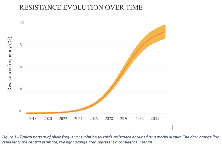
Resistance-evolution models have a limited prediction power, but within the boundaries defined in the model itself, researchers can take advantage of a large number of simulations to provide probabilistic predictions (e.g. “within the limits of this model, we can predict that resistance that resistance frequency can reach 50% in 5 to 10 years, with 95% confidence”). Just as weather forecast, there is a chance that the prediction will not realise. Still weather forecasts are an incredibly useful tool used everywhere in the world.
The main advantage of predictive models in this context, however, is the possibility of comparing alternative scenarios (strategies) and evaluate their relative performance. Even if the absolute numbers are not necessarily spot on, the comparison of alternative scenarios tends to be very reliable in determining the better resistance-management strategy to be implemented in real life.
Are all insecticide resistance simulation models the same? If not, what are the differences?
Computational models differ in several aspects; and models for insecticide resistance evolution are no exception. The first aspect in which models can vary is the level of granularity in which they are built (in other words, how many parameters/variables are required to regulate the process under scrutiny): A model can set about describing high-level general patterns of population density, for instance. To investigate phenomena at this level, simple models including a handful of variables are probably enough. Models which would involve population density plus interaction with the environment would need additional parameters, including interaction parameters.
There are also different schools of modelling and they have a relation with the level of granularity in which researchers are interested in exploring:
Some models, in fact, don’t even require simulations to be run as their components can be sufficiently well described by a series of equations, which in turn can be solved analytically. Slightly more complex models still involve a series of equations, but they can be tricky enough to require computational methods to be solved. These are the equation-based models, which tend to investigate a problem in top-down manner.
Agent- or individual-based models (IBMs) come from a different school of thought: They are built bottom-up, where their more fundamental parts are the individual agents in the system (e.g. insects in the pest population). The complexity of a model like this depends on how many levels the model contains (e.g. individuals (1) that form a population (2), possibly part of meta-population (3 levels)) and the number of variables each individual contains (e.g. sex, age, feeding behaviour, number of populations, population size, etc.). This kind of model almost always requires computer simulations to come to life and has only been used to extent in which computers can handle them, of course.
Regardless of the school of modelling used, simplicity is always the order of the day. A good model is only as complex as necessary (not a single parameter more).
Different questions in insecticide resistance evolution can be better tackled in either one or other approach. If simple and well-known high-level phenomena are the focus, equation-based models are generally all that is needed; if there are more low-level nuances to the question and emergent properties of the system could be expected, then IBMs tend to provide more robust depictions of the real-world system.
What kind of information do I need to build an insecticide resistance simulation model?
This depends heavily on the kind of model chosen (see question above), but a typical resistance evolution model would incorporate the following information:
- Fundamental pest-biology parameters
- Population dynamics
- Population size – This is a key number defining the kind of evolutionary processes a population will undergo. The lower the population size, the higher the odds of stochastic events to happen (genetic drift). Larger population sizes, in turn, lead to more deterministic processes involving natural selection.
- Reproductive biology – The way insects go through their life cycles varies dramatically. These differences need to be accounted for with parameters defining their life stages, their mode of reproduction and their reproductive potential.
- Natural mortality – The majority of insect species have their populations naturally controlled by biotic and environmental phenomena (e.g. resource availability, predation, seasonal temperature variations, etc.). Pest insects are also subject to these phenomena, but to different extents in different situations.
- Migration rate – The ability of genes to spread across populations is regulated by the migration rate in the meta-population. The higher its value, the more rapidly a resistant mutation will spread in space.
- Genetics
- Resistance factor – This parameter works as a summary of complex underlying biochemical processes that determine how much more successful resistant individuals are when compared to susceptible ones. The more relatively successful a resistant form is, the more quickly it will tend to dominate the population.
- Standing resistance-allele frequency – This determines how common resistant forms are before the population is exposed to the treatment (either by standing genetic variation or mutation). If resistant forms are common, pest resistance will emerge more rapidly.
- Other genetic factors – The genetics of adaptation can be very complex, involving multiple genes, modes of inheritance, degrees of expression, and dominance within and between loci. Models for resistance evolution normally assume the simplest case (one gene with two forms), but researchers are investigating what consequences deviations from this case can have in the final outcome (i.e. time to resistance).
- Fundamental crop-protection parameters
- Baseline efficacy of the product(s) against different pest life stages – The efficacy (strength) of an insecticide combined with the resistance factor (above) determines the selective force applied to the population. An insect that is resistant to a strong product will have relatively more reproductive success than an insect resistant to a weaker insecticide, when compared to the respective susceptible forms.
- Crop protection strategy (e.g. product alternations and mixtures, crop(s) – This characteristic of a model aggregates as series of parameters related to how the pest control is carried out. It is precisely at this point that different scenarios can be devised and compared to find the more adequate solutions to keep resistance at bay.
- Additional parameters
- Weather – Weather has direct effects on the biology of both pest and crop. It is important to account for weather variation when providing resistance-evolution predictions.
- Crop-pest interactions – A crop may provide different levels of support to a pest population depending on its development stage and variety. This translates into different maximum population sizes for the pest, which affects directly the first parameter discussed in this list (above).
- Landscape parameters (e.g. proportion of crop fields, nature and other areas) – Evolution of resistance happens in time and space. The time frame to be investigated is generally clear and straightforward (e.g. 25 or 50 years); the space can vary dramatically in size and composition. Models often include different scenarios for the latter (e.g. field mosaics), whereas the total area is generally as large as what can be treated with current computational power, especially with individual-based models.
- Population dynamics
Modelling evolutionary processes is a complex undertaking and doing that for evolution of pesticide resistance is no exception. Therefore a good deal of modelling expertise combined with a deep understanding of evolution and agronomy is required to build sensible models and to make sense of their results. The effort is worthwhile, though: Modelling can provide much more precise and potentially accurate results, which can be directly translated into resistance management recommendations tailor-made for every situation.
To learn more
Bourguet, D., F. Delmotte, P. Franck, T. Guillemaud, X. Reboud, C. Vacher, and A. S. Walker. 2010. The skill and style to model the evolution of resistance to pesticides and drugs. Evolutionary Applications 3:375–390.
Gould, F., Z. S. Brown, and J. Kuzma. 2018. Wicked evolution: Can we address the sociobiological dilemma of pesticide resistance? Science 360:728–732.
Roff, D. A. 2010. Modelling Evolution. Oxford University Press.
Roush, R. T. 1993. Occurrence, Genetics and Management of Insecticide Resistance. Parasitology Today 9:174–179.
South, A., and I. M. Hastings. 2018. Insecticide resistance evolution with mixtures and sequences: A model-based explanation. Malaria Journal 17:1–20.
South & Hastings’s online interactive model: https://andysouth.shinyapps.io/resistmixseq/